Mean-centred analysis of volume source data

This example demonstrates how we to use mean-centred PLS to identify condition-wise differences in source time courses in a volumetric source space.

Loading data

We will begin by loading the sample data and extracting epochs corresponding to auditory stimuli presented to the left versus right ear.

import mne
from mne.datasets import sample
from mne.minimum_norm import apply_inverse, apply_inverse_epochs, read_inverse_operator
import mne_plsc

data_path = sample.data_path()
meg_path = data_path / "MEG" / "sample"
fname_raw = meg_path / "sample_audvis_filt-0-40_raw.fif"
fname_event = meg_path / "sample_audvis_filt-0-40_raw-eve.fif"

# Load data
raw = mne.io.read_raw_fif(fname_raw)
events = mne.read_events(fname_event)

# pick MEG channels
picks = mne.pick_types(
    raw.info, meg=True, eeg=False, stim=False, eog=True, exclude="bads"
)
# Read epochs
epochs = mne.Epochs(
    raw,
    events,
    event_id={'left': 1, 'right': 2},
    tmin=-0.2, tmax=0.5,
    picks=picks,
    baseline=(None, 0),
    reject=dict(mag=4e-12, grad=4000e-13, eog=150e-6),
    preload=True,
    verbose=False
)
# Crop to a small window for speed
epochs = epochs.crop(tmin=0.05, tmax=0.1)

Opening raw data file /home/docs/mne_data/MNE-sample-data/MEG/sample/sample_audvis_filt-0-40_raw.fif...
    Read a total of 4 projection items:
        PCA-v1 (1 x 102)  idle
        PCA-v2 (1 x 102)  idle
        PCA-v3 (1 x 102)  idle
        Average EEG reference (1 x 60)  idle
    Range : 6450 ... 48149 =     42.956 ...   320.665 secs
Ready.

Computing volume source estimate

Next, we will load the pre-computed inverse operator for the sample dataset and apply it to the epochs. This yields a list of source time courses (STCs).

fname_inv = meg_path / "sample_audvis-meg-vol-7-meg-inv.fif"
inverse_operator = read_inverse_operator(fname_inv, verbose=False)

snr = 3.0
lambda2 = 1.0 / snr**2
stcs = apply_inverse_epochs(
    epochs=epochs,
    inverse_operator=inverse_operator,
    lambda2=lambda2,
    method='dSPM',
    verbose=False
)

Fitting and assessing mean-centred PLS model

Next, we will get the labels for the epochs and use them to fit a mean-centred PLS model. In order to render a 4D image of the brain saliences, we will attach info about the source space to the model. For a volumetric source space, this means adding the VolSourceSpaces object corresponding to the inverse operator.

labels = mne_plsc.utils.get_epoch_labels(epochs)
res = mne_plsc.fit_mc(stcs,
                      between=labels,
                      random_state=123)
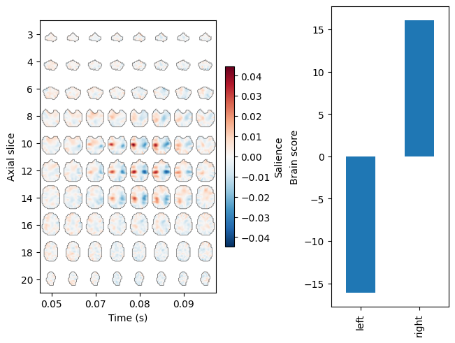
res.add_source_info(src=inverse_operator['src'])
res.plot_lv(0)

Assuming time-domain source-space data. If data is actually freq- or time-freq-domain, specify this explicitly

(<Figure size 640x480 with 3 Axes>,
 array([<Axes: xlabel='Time (s)', ylabel='Axial slice'>,
        <Axes: ylabel='Brain score'>], dtype=object))

We can assess the significance of the model using permutation testing. We will do a small number of permutations here for speed, but for real data it would be best to do many more.

res.permute(100)
print(res.summary())

Getting permutations: 100%|██████████| 100/100 [00:00<00:00, 122712.23it/s]
Permuting: 100%|██████████| 100/100 [00:00<00:00, 238.41it/s]

   LV index  singular value  variance explained   p value
0         0       22.784547                 1.0  0.009901
1         1        0.000000                 0.0       NaN

Thus, the model has identified a significant contrast between the conditions.

Cluster analysis

To characterize the pattern that differentiates the two conditions, we can perform cluster analysis. First, we will perform bootstrap resampling to estimate the \(z\) scores of the brain saliences.

res.bootstrap(100)

Getting resamples: 100%|██████████| 100/100 [00:00<00:00, 6954.00it/s]
Resampling: 100%|██████████| 100/100 [00:00<00:00, 108.04it/s]

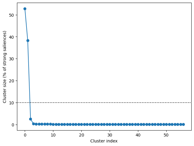
Next, we can add an adjacency matrix and compute clusters. Computing adjacency requires adding source info (via add_source_info), which we did before. As the plot below shows, there are two major clusters in the data—each other cluster accounts for less than 10% of the strong saliences.

res.add_adjacency()
res.cluster(threshold=3)
f, ax = res.plot_cluster_sizes(lv_idx=0)
ax.axhline(y=10, c='k', ls=':')

-- number of adjacent vertices : 3757
Clustering z-scores
Defaulting to unsigned clustering
Computing clusters for lv_idx 0...
Threshold: 3
57 clusters

<matplotlib.lines.Line2D at 0x7312e9fa8f50>

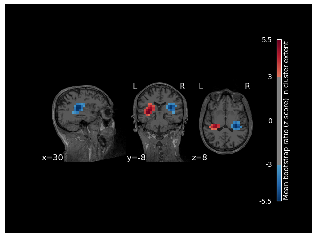
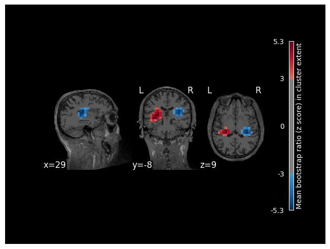
To visualize clusters, we will attach the subject’s MRI to the model (which will then be used as a background image). Visualizing these first two clusters, we can see that they overlap with the left and right auditory cortex.

res.add_source_info(mri=data_path / "subjects" / "sample" / "mri" / "T1.mgz")
res.plot_cluster_spatial(lv_idx=0, cluster_idx=0, highlight='extent')
res.plot_cluster_spatial(lv_idx=0, cluster_idx=1, highlight='extent')

(<Figure size 640x480 with 5 Axes>, <Axes: >)