Mean-centred analysis of surface source-space data

This notebook will illustrate how to identify condition-wise differences in (surface) source-space data using mean-centred PLS.

Getting source-space data

import mne
from mne.datasets import sample
from mne.minimum_norm import apply_inverse_epochs, read_inverse_operator
import mne_plsc

data_path = sample.data_path()
meg_path = data_path / "MEG" / "sample"
fname_inv = meg_path / "sample_audvis-meg-oct-6-meg-inv.fif"
fname_raw = meg_path / "sample_audvis_filt-0-40_raw.fif"
fname_event = meg_path / "sample_audvis_filt-0-40_raw-eve.fif"

# Load data
inverse_operator = read_inverse_operator(fname_inv)
raw = mne.io.read_raw_fif(fname_raw)
events = mne.read_events(fname_event)

# Add a bad channel
raw.info["bads"] += ["EEG 053"]  # bads + 1 more

# Create epochs
picks = mne.pick_types(
    raw.info, meg=True, eeg=False, stim=False, eog=True, exclude="bads"
)
epochs = mne.Epochs(
    raw,
    events,
    event_id={'left': 1, 'right': 2},
    tmin=-0.2, tmax=0.5,
    picks=picks,
    baseline=(None, 0),
    reject=dict(mag=4e-12, grad=4000e-13, eog=150e-6),
    preload=True,
    verbose=False
)

# Crop to small time window for speed
epochs.crop(0.05, 0.1)

# Apply inverse operator
snr = 3.0
lambda2 = 1.0 / snr**2
method = "dSPM"
stcs = apply_inverse_epochs(
    epochs,
    inverse_operator,
    lambda2,
    method,
    pick_ori="normal",
    verbose=False
)

Reading inverse operator decomposition from /home/docs/mne_data/MNE-sample-data/MEG/sample/sample_audvis-meg-oct-6-meg-inv.fif...
    Reading inverse operator info...
    [done]
    Reading inverse operator decomposition...
    [done]
    305 x 305 full covariance (kind = 1) found.
    Read a total of 4 projection items:
        PCA-v1 (1 x 102) active
        PCA-v2 (1 x 102) active
        PCA-v3 (1 x 102) active
        Average EEG reference (1 x 60) active
    Noise covariance matrix read.
    22494 x 22494 diagonal covariance (kind = 2) found.
    Source covariance matrix read.
    22494 x 22494 diagonal covariance (kind = 6) found.
    Orientation priors read.
    22494 x 22494 diagonal covariance (kind = 5) found.
    Depth priors read.
    Did not find the desired covariance matrix (kind = 3)
    Reading a source space...
    Computing patch statistics...
    Patch information added...
    Distance information added...
    [done]
    Reading a source space...
    Computing patch statistics...
    Patch information added...
    Distance information added...
    [done]
    2 source spaces read
    Read a total of 4 projection items:
        PCA-v1 (1 x 102) active
        PCA-v2 (1 x 102) active
        PCA-v3 (1 x 102) active
        Average EEG reference (1 x 60) active
    Source spaces transformed to the inverse solution coordinate frame
Opening raw data file /home/docs/mne_data/MNE-sample-data/MEG/sample/sample_audvis_filt-0-40_raw.fif...
    Read a total of 4 projection items:
        PCA-v1 (1 x 102)  idle
        PCA-v2 (1 x 102)  idle
        PCA-v3 (1 x 102)  idle
        Average EEG reference (1 x 60)  idle
    Range : 6450 ... 48149 =     42.956 ...   320.665 secs
Ready.

Fitting and assessing model

First, we will extract the epoch labels and use them to fit a mean-centred model. Then we will assess the significance of the model using permutation testing. We will do a small number of permutations for speed here; a real analysis requires many more.

labels = mne_plsc.utils.get_epoch_labels(epochs)
res = mne_plsc.fit_mc(data=stcs,
                      between=labels)
res.permute(100)
print(res.summary())

Assuming time-domain source-space data. If data is actually freq- or time-freq-domain, specify this explicitly

Getting permutations: 100%|██████████| 100/100 [00:00<00:00, 150819.99it/s]
Permuting: 100%|██████████| 100/100 [00:01<00:00, 98.61it/s]

   LV index  singular value  variance explained   p value
0         0       57.759548                 1.0  0.009901
1         1        0.000000                 0.0       NaN

As we can see, the model has identified a pattern differentiating between the left and right ear auditory conditions.

Cluster analysis

To characterize the spatial and temporal distribution of the pattern that differentiates the conditions, we can do cluster analysis. For this, we first need to add information about the source space: both the SourceSpaces object corresponding to the inverse operator and the freesurfer subjects directory. After this, we can add an adjacency matrix and identify clusters. Here we will perform clustering on the raw saliences and skip bootstrap resampling for speed.

res.add_source_info(src=inverse_operator['src'],
                    subjects_dir=data_path / 'subjects')
res.add_adjacency()
res.cluster(threshold=0.01)

-- number of adjacent vertices : 8196

/tmp/ipykernel_1148/2578940426.py:3: RuntimeWarning: 8.5% of original source space vertices have been omitted, tri-based adjacency will have holes.
Consider using distance-based adjacency or morphing data to all source space vertices.
  res.add_adjacency()

Clustering saliences
Defaulting to unsigned clustering
Computing clusters for lv_idx 0...
Threshold: 0.01
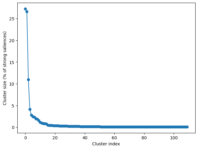
110 clusters

As we can see, there are two major clusters:

res.plot_cluster_sizes(lv_idx=0)

(<Figure size 640x480 with 1 Axes>,
 <Axes: xlabel='Cluster index', ylabel='Cluster size (% of strong saliences)'>)

Visualizing clusters

We can visualize these clusters using the plot_cluster_spatial() method, which produces and interactive 3D rendering. This is not possible in a static HTML notebook, so it has to be run on your own computer.

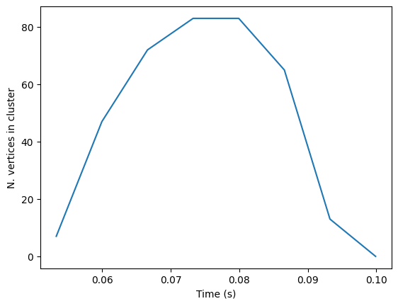
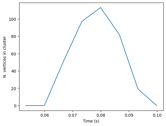
However, we can still see the temporal distribution of the clusters:

res.plot_cluster_nonspatial(lv_idx=0, cluster_idx=0)
res.plot_cluster_nonspatial(lv_idx=0, cluster_idx=1)

(<Figure size 640x480 with 1 Axes>,
 <Axes: xlabel='Time (s)', ylabel='N. vertices in cluster'>)